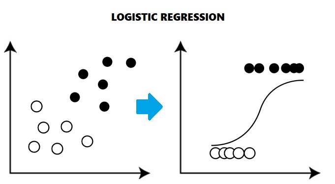
Understanding Logistic Regression
Introduction
Companies need to make data – led decisions. Often these decisions have simple Yes or No outcomes. In Data parlance we call this a Binary outcome. Some examples of this can be as below
- Will recipients open our Marketing Email OR Not?
- Is an E-mail Spam or Not?
- Should we give an applicant a loan or Not?
Basically, we need a logical method or an algorithm to classify the E-mail or applicant into one or two categories. But how do we do this, as there are many factors influencing the ‘Yes’ or ‘No’ decision or the binary outcome. In another words the outcome is a varies or depends on many other variables. The answer to these problems is Logistic regression.
A sample problem
Let’s take an example of whether an e-mail will be labelled as Spam or not to learn the important terms. Whether an e-mail is spam or not can depend on many factors which are also called Independent Variables:
- Whether the site sending it is secure or not
- The number of links in the email
- The kind of attachments in the email
- Whether other users have flagged that e-mail as spam
- The IP Address of the sender
In this case the whether the E-mail is opened or not is the dependent variable as it depends on variables like the five listed above.
Terms used in Logistic Regression
Technically, Logistic regression is a machine learning classification algorithm. It helps us to find the chances of probability of a categorical dependent variable like an E-mail being labelled Spam or not with the help of logistic functions.
The outcome of logistic regression is any binary value such as Male or Female, Yes or No, 1 or 0, Spam or Not Spam. Nowadays it is widely used for classifying things. There are many examples which are evident that machine learning algorithms have made our lives easier as an accurate Logistics regression model helps us take decisions faster once it has been trained on training data.
Training data is the data that the algorithm learns from. It contains sample values of dependent and independent variables that the algorithm can be trained on. Once it is trained it can be checked on the test data. This is a new data set that the algorithm is exposed to see if it can make accurate predictions.
Business Case Study
Case Study Santam Insurance saves $2.4 million using Analytics
The South African Insurance Company Santam used Analytics to process the insurance claims and determine if they are fraudulent or not. This is a clear Logistics Regression problem. It enabled Santam to make faster payouts for legitimate claims and reduce losses on fraudulent claims.
Se we see Logistic regression increased the speed and efficiency of the processing methodologies and improved the customer experience. Santam sets a wonderful example how the companies can protect their business from frauds as well as customers from being deceived. Another benefit was that they were able to reduce the on the ground investigators, evaluator and workforce that would manually investigate claims for genuineness.

How does Logistic regression work?
Logistic regression uses functions called the logit functions to derive a relationship between the dependent variable and independent variables by estimating the best probabilities or chances of occurrence.
The logistic functions (also known as the sigmoid functions) convert the probabilities into binary values which could be further used for predictions.

Logit Functions – Don’t worry if it looks mathematical
Logistic regression is the estimate of the logit functions which could be calculated as the logarithm of the odd ratios. There are simple functions that help us do this in Excel, R or Python. Or we can also use the formula for the function.

This is the simple logistic regression equation for prediction of probability of the occurrence of interested outcome
Log-Likelihood Function
The Log-Likelihood function is as below. This is the function that gives us the final likely hood or result. Such as to give the loan or not. This is the final output we desire of the Logistic regression model.
LL = ∑ Yi*P(Xi) + (1 – Yi)(1 – P(Xi))
Advantages
- It is easy to implement and very efficient to train.
- Because of its simplicity it can be implemented quickly.
Disadvantages
It cannot solve non-linear problems or problems where we can’t use a line to plot the relationship between variables.
It needs all of its independent variables to be identified properly. This can be a big task in a business where there are 300+ variables in the data and additionally macroeconomic factors such as inflation, dollar exchange rates etc.
Logistic regression using Excel
We have dataset of 20 similar machines and we want to predict if all of them produce output as per our specifications.
| Machine
meets Specification |
Machine
Age (Months) |
Average
Number of shifts per week |
| 1 | 57 | 4 |
| 0 | 73 | 5 |
| 1 | 22 | 5 |
| 0 | 59 | 4 |
| 1 | 15 | 4 |
| 1 | 36 | 2 |
| 0 | 68 | 5 |
| 0 | 49 | 5 |
| 0 | 27 | 7 |
| 1 | 59 | 3 |
| 1 | 10 | 6 |
| 0 | 78 | 8 |
| 1 | 22 | 6 |
| 1 | 36 | 4 |
| 0 | 57 | 7 |
| 0 | 73 | 8 |
| 1 | 38 | 5 |
| 0 | 71 | 7 |
| 0 | 35 | 4 |
| 1 | 44 | 5 |
We have assumed our binary output in the following manner: –
1 – Machine meets the specifications
0 – Machine does not meet the specifications
Step 1– First we will sort our data
Using excel sorting tool just sort the data on the basis of dependent variable.
| Machine
meets Specification |
Machine
Age (Months) |
Average
Number of shifts per week |
| 0 | 78 | 8 |
| 0 | 73 | 8 |
| 0 | 73 | 5 |
| 0 | 71 | 7 |
| 0 | 68 | 5 |
| 0 | 59 | 4 |
| 0 | 57 | 7 |
| 0 | 49 | 5 |
| 0 | 35 | 4 |
| 0 | 527 | 7 |
| 1 | 59 | 3 |
| 1 | 57 | 4 |
| 1 | 44 | 5 |
| 1 | 38 | 5 |
| 1 | 36 | 4 |
| 1 | 36 | 2 |
| 1 | 22 | 6 |
| 1 | 22 | 5 |
| 1 | 15 | 4 |
| 1 | 10 | 6 |
Step 2– Calculating Logit Function
We will have a logit function with explanatory variables as Age and Average number of shifts
L = b0 + b1*Age + b2*Average number of shifts
We will take arbitrary values for bo, b1 and b2 as 0.1
Now we will calculate the L (logit function) value for the data
| Machine
meets Specification |
Machine
Age (Months) |
Average
Number of shifts per week |
Logit values
(L) |
| 0 | 78 | 8 | 8.7 |
| 0 | 73 | 8 | 8.2 |
| 0 | 73 | 5 | 7.9 |
| 0 | 71 | 7 | 7.9 |
| 0 | 68 | 5 | 7.4 |
| 0 | 59 | 4 | 6.4 |
| 0 | 57 | 7 | 6.5 |
| 0 | 49 | 5 | 5.5 |
| 0 | 35 | 4 | 4 |
| 0 | 527 | 7 | 3.5 |
| 1 | 59 | 3 | 6.3 |
| 1 | 57 | 4 | 6.2 |
| 1 | 44 | 5 | 5 |
| 1 | 38 | 5 | 4.4 |
| 1 | 36 | 4 | 4.1 |
| 1 | 36 | 2 | 3.9 |
| 1 | 22 | 6 | 2.9 |
| 1 | 22 | 5 | 2.8 |
| 1 | 15 | 4 | 2 |
| 1 | 10 | 6 | 1.7 |
Step 3– Calculate P(x) for each data record
P(x) =eL /(1 + eL)
| Machine
meets Specification |
Machine
Age (Months) |
Average
Number of shifts per week |
Logit values
(L) |
eL | P(x) |
| 0 | 78 | 8 | 8.7 | 6002.912247 | 0.990833442 |
| 0 | 73 | 8 | 8.2 | 3630.950324 | 0.999725422 |
| 0 | 73 | 5 | 7.9 | 2697.28234 | 0.999629394 |
| 0 | 71 | 7 | 7.9 | 2697.28234 | 0.999629394 |
| 0 | 68 | 5 | 7.4 | 1635.984437 | 0.999389121 |
| 0 | 59 | 4 | 6.4 | 601.8450401 | 0.998341199 |
| 0 | 57 | 7 | 6.5 | 665.1416355 | 0.998498818 |
| 0 | 49 | 5 | 5.5 | 244.691933 | 0.995929862 |
| 0 | 35 | 4 | 4 | 54.59815016 | 0.98201379 |
| 0 | 527 | 7 | 3.5 | 33.11545202 | 0.970687769 |
| 1 | 59 | 3 | 6.3 | 544.5719121 | 0.998167061 |
| 1 | 57 | 4 | 6.2 | 492.7490428 | 0.99797468 |
| 1 | 44 | 5 | 5 | 148.4131595 | 0.993307149 |
| 1 | 38 | 5 | 4.4 | 81.45086887 | 0.987871565 |
| 1 | 36 | 4 | 4.1 | 60.34028774 | 0.983697501 |
| 1 | 36 | 2 | 3.9 | 49.40244921 | 0.980159694 |
| 1 | 22 | 6 | 2.9 | 18.1741454 | 0.947846437 |
| 1 | 22 | 5 | 2.8 | 16.4446468 | 0.942675824 |
| 1 | 15 | 4 | 2 | 7.389056107 | 0.880797078 |
| 1 | 10 | 6 | 1.7 | 5.473947397 | 0.845534735 |
Step4- Calculating Log-Likelihood Function
We will now calculate the values
| -8.700166577 |
| -8.200274621 |
| -7.900370679 |
| -7.900370679 |
| -7.40061107 |
| -6.401660182 |
| -6.501502314 |
| -5.504078446 |
| -4.01814993 |
| -3.52975042 |
| -0.001834621 |
| -0.002027374 |
| -0.006715348 |
| -0.012202585 |
| -0.016436847 |
| -0.020039767 |
| -0.053562776 |
| -0.059032826 |
| -0.126928011 |
| -0.167786029 |
Step5- Calculating Maximum Log-Likelihood Function
Earlier we assumed the value of the coefficients for our logit function. Now we will find those values of coefficients which maximize our log-likelihood function.
For this purpose we will use an Excel tool that is Excel Solver. Its purpose is to adjust the numeric value in a particular cell so that we could maximize or minimize the value in desired cells.
We will take columns 2, 3 and 4 for evaluation.
After running the Excel Solver we will get the following output. According to this new values of coefficient will be b0, b1 and b2.
| bo | 12.48285608 |
| b1 | -0.117031374 |
| b2 | -1.469140055 |
Values of all log-likelihood will change according to the values of b0, b1, and b2.
The new value of maximum log-likelihood (summation of all log-likelihood) will be: – -6.654560484.
Step6– Evaluate values
For any values of age and average number of shifts you can predict the probabilities using the new values of coefficients.
In this case the probability of the desired output being produced by the Machine is only 8% which is very low. Now, co-relation is not causation so we cannot blame this on Age and weekly shifts alone. In a full blown Logistic regression model, we would have many more variables and accuracy.

Similarly, the other values show that the logit function is consistent with the given data. Hence we can predict any probability with this equation with the help of excel solver.
You may also like
